

Fabian, a 15-year-old school intern, worked on a Monte Carlo simulation project using one of our HIFIS Jupyter Services. During his three-week internship, he focused on three key areas:
- understanding the CMS Detector and producing interactive plots in Jupyter notebook,
- exploring B Meson Decay and making a short animation,
- and simulating parton transverse momentum distribution using PYTHIA.
His work yielded valuable results, showcasing how HIFIS can support projects, even at the high school level. It allowed Fabian and his supervisors to dive directly into the research with minimal overhead. This straightforward use case exemplifies a frequent need in both educational and research settings.
Let us dig a bit deeper in the notebook with one example.
Exploring B Meson Decay
The B meson decay is a process where a heavy particle breaks down into lighter ones, following the weak interaction. It first decays into a D meson, a muon, and a neutrino. The D meson then decays into a kaon and a pion, while the pion can further decay into another muon and neutrino. Studying these decays helps physicists understand quark transitions, test the Standard Model, and explore CP violation*, which may explain why the universe favors matter over antimatter.
Here’s a code snippet from Fabian’s notebook that illustrates this decay process using a Sankey diagram:
1
2
3
4
5
6
7
8
9
10
11
12
13
14
15
16
17
18
19
20
21
22
23
24
25
26
27
28
29
30
31
32
33
34
import plotly.graph_objects as go

# Define particles in the decay chain (realistic version)
particles = ['B Meson', 'D Meson', 'Muon', 'Neutrino', 'Kaon', 'Pion']

# Define how particles are connected (what decays into what)
decays = [
    ('B Meson', 'D Meson'),
    ('B Meson', 'Muon'),
    ('B Meson', 'Neutrino'),
    ('D Meson', 'Kaon'),
    ('D Meson', 'Pion'),
    ('Pion', 'Muon'),
    ('Pion', 'Neutrino')
]

# Create the diagram
fig = go.Figure(go.Sankey(
    node=dict(
        pad=15,
        thickness=20,
        line=dict(color='black', width=0.5),
        label=particles  # The names of particles
    ),
    link=dict(
        source=[particles.index(source) for source, _ in decays],  # Where the decay starts
        target=[particles.index(target) for _, target in decays],  # Where the decay goes
        value=[1 for _ in decays],  # The strength of each decay (simplified to 1)
    )
))

# Add title and show the diagram
fig.update_layout(title_text="Corrected B Meson Decay Chain", font_size=14)
fig.show()
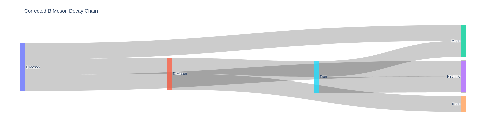
While this static plot effectively illustrates the primary decay channels, it omits additional possible decay channels and intermediate particles. For example, the D meson can decay in multiple ways, not just into a kaon and pion. By reproducing the entire Sankey chart using the code snippet above, you can visualise the B Meson decay chain interactively, and modify the structure to represent different decay scenarios or branching probabilities.
*CP violation is a phenomenon where the laws of physics behave differently for particles and their corresponding antiparticles when their spatial coordinates are inverted. More on this from CERN.
Get in contact
If a similar need arises on your side, you can explore our HIFIS Jupyter Services. Should any question come up along the way, reach out to us at HIFIS Support.