Matplotlib Fundamentals

Overview¶

Let’s take a look at matplotlib first. We will introduce the required technical terms to better understand how the framework conceptualizes the stucture of a plot. Afterwards we will create our first very own plot with Python.

Anatomy of a Plot¶

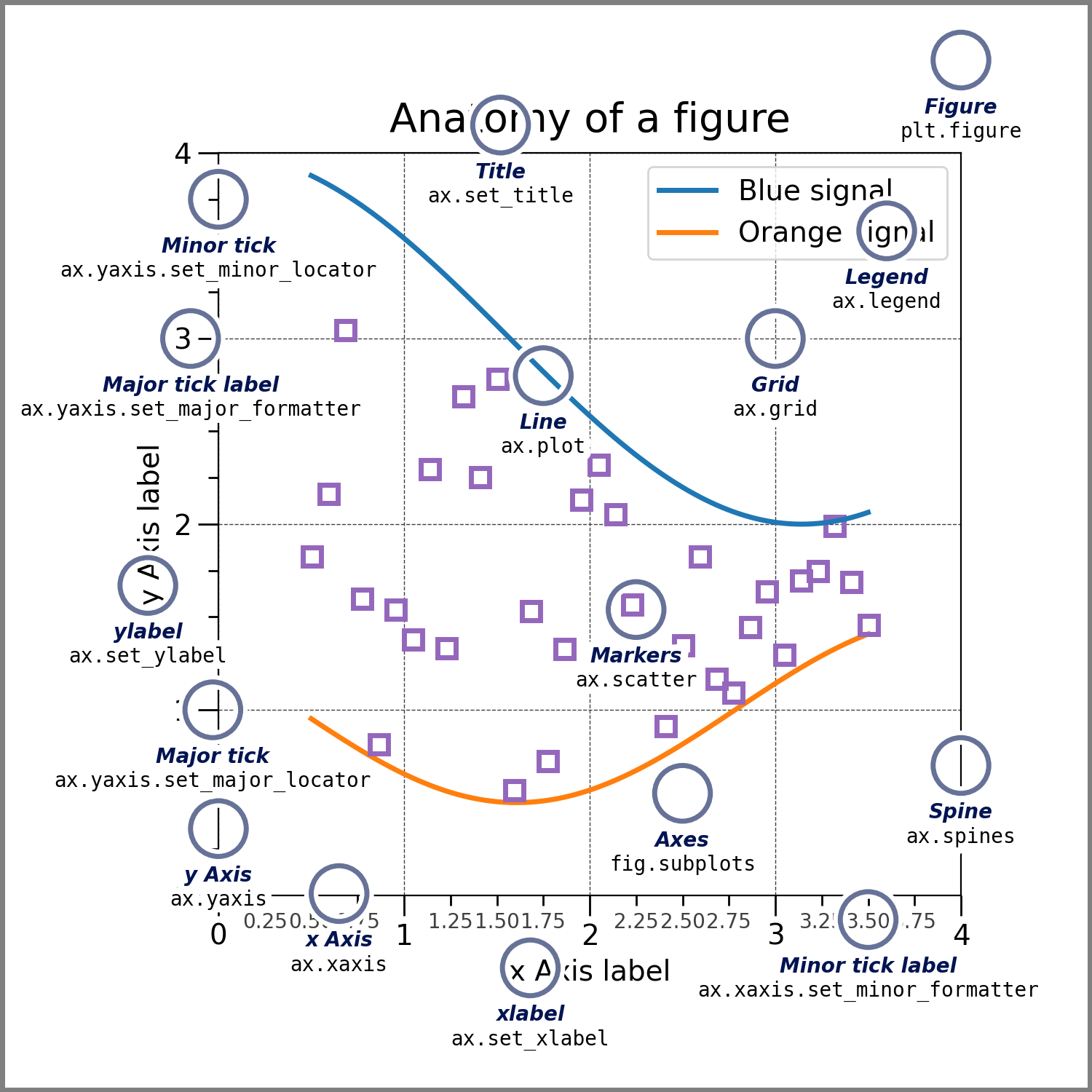
For understanding how matplotlib names the various elements, we can take a look at this sketch from the official documentation.

Example plot with elements labelled

Easy to get confused

There are two terms that sound very similar and can be easily confused:

Axis: the number line that gets printed on the side of the plot
Axes: the collection of all plotted elements that represent data (roughly: the plotting area)

Creating a simple Plot¶

We start by creating a new python script, called simple_plot.py.

Example Data¶

For demonstrating how to use matplotlib, we need some data to actually plot. We are going to use some temperature measurements as an example:

simple_plot.py

# Measured air temperature in °C
# Central Park, New York, US 
# 2020-12-31, 00:00 - 23:00

air_temperature = [
    5.0, 5.6, 5.6, 5.6, 5.6, 6.1, 6.7, 7.2,
    7.8, 8.3, 8.3, 8.9, 7.8, 7.2, 7.2, 7.2,
    6.7, 6.7, 6.7, 6.7, 6.1, 5.6, 5.0, 5.0
]

The first Steps¶

The matplotlib framework offers a collection of shortcuts in the pyplot module. We can import this module and use the functions it offers to quickly create a fundamental plot. We have to do two steps:

Generating the actual plot
Showing this new plot to the user

simple_plot.py

from matplotlib import pyplot

# Measured air temperature in °C
# Central Park, New York, US 
# 2020-12-31, 00:00 - 23:00

air_temperature = [
    5.0, 5.6, 5.6, 5.6, 5.6, 6.1, 6.7, 7.2,
    7.8, 8.3, 8.3, 8.9, 7.8, 7.2, 7.2, 7.2,
    6.7, 6.7, 6.7, 6.7, 6.1, 5.6, 5.0, 5.0
]

pyplot.plot(air_temperature)
pyplot.show()

pyplot keeps track

The pyplot module internally keeps track of how the state of the plot changes based on the functions you called. This allows you to create a plot step-by-step without worrying about bookkeeping each part of the plot. Once you show the plot, pyplot will forget about the state and is ready to start from scratch.

Adding Details¶

This basic plot lacks many of the details that we are used to seeing on a proper data presentation. Let’s improve by adding some values for the x-axis.

Since we are dealing with dates and times, it would be a good idea to refer to Pythons’ built-in datetime module for now.

simple_plot.py

from matplotlib import pyplot
from datetime import datetime, timedelta

# Measured air temperature in °C
# Central Park, New York, US 

start_time = datetime(year=2020, month=12, day=31, hour=0)
air_temperature = [
    5.0, 5.6, 5.6, 5.6, 5.6, 6.1, 6.7, 7.2,
    7.8, 8.3, 8.3, 8.9, 7.8, 7.2, 7.2, 7.2,
    6.7, 6.7, 6.7, 6.7, 6.1, 5.6, 5.0, 5.0
]

hours = [
    start_time + timedelta(hours=offset) 
    for offset in range(len(air_temperature))
]

pyplot.plot(hours, air_temperature)
pyplot.show()

Providing x- and y-data to plot()

To plot a curve a sequence of x-y-coordinates is required. In matplotlib these are given as separate sequences for x-components and y-components. To form the actual coordinates, the sequence elements will be matched in order.

When only providing one argument to the plot()-function, pyplot automatically assumes that these are the coordinate components on the y-axis and that their indices are the matching coordinate components on the x-axis.

If two sequences are provided, it is instead assumed that the first sequence will hold the x-axis components and the second sequence holds the y-axis components.

More information and examples can be found in the plot()-function documentation

Our current plot has just the bare essentials and still could use some fine tuning before it becomes paper-worthy. Let’s start our improvements by adding some proper labels to the axis and a title.

simple_plot.py

from matplotlib import pyplot
from datetime import datetime, timedelta

start_time = datetime(year=2020, month=12, day=31, hour=0)
air_temperature = [
    5.0, 5.6, 5.6, 5.6, 5.6, 6.1, 6.7, 7.2,
    7.8, 8.3, 8.3, 8.9, 7.8, 7.2, 7.2, 7.2,
    6.7, 6.7, 6.7, 6.7, 6.1, 5.6, 5.0, 5.0
]

hours = [
    start_time + timedelta(hours=offset) 
    for offset in range(len(air_temperature))
]

pyplot.title("Central Park, New York, US")
pyplot.xlabel("Local time")
pyplot.ylabel("Air Temperature [°C]")

pyplot.plot(hours, air_temperature)
pyplot.show()

By default, pyplot will try its best to fit the plotted data smoothly into the given drawing area and then determines where to put the tick marks from that. We can fine-tune this behaviour by manually setting the limits, values and labels for the tick marks.

Common Misconception

Setting the labels of tick marks does not change their value. Functions that require the data points for orientation (e.g. tick marks, marker lines, filling areas) will still require the underlying values to work properly. Changing the labels is purely for visual presentation.

Example: pyplot.xticks() requires the ticks parameter, indicating where markers are to be placed. These ticks must be a subset of the x-valued provided to plot() earlier. You may also pass a labels parameter, indicating how the individual ticks are supposed to be represented. These labels can be chosen freely and will be associated with the ticks in order.

While in our case the y-axis looks pretty fine, we will have to work on the x-axis a bit. Let’s improve it by doing the following:

Make more room on the axis by only printing a tick for every second hour
Rotate them by 45° to fit better when close together
- Use the right side as the rotation point, so the rotated text aligns nicely with the tick marks
- Since matplotlib considers labels as text objects, you can use all associated text properties
Format the labels as HH:MM (i.e. two-digit hours and minutes)
- See the strftime() documentation for details on the formatting

simple_plot.py

from matplotlib import pyplot
from datetime import datetime, timedelta

start_time = datetime(year=2020, month=12, day=31, hour=0)
air_temperature = [
    5.0, 5.6, 5.6, 5.6, 5.6, 6.1, 6.7, 7.2,
    7.8, 8.3, 8.3, 8.9, 7.8, 7.2, 7.2, 7.2,
    6.7, 6.7, 6.7, 6.7, 6.1, 5.6, 5.0, 5.0
]

hours = [
    start_time + timedelta(hours=offset) 
    for offset in range(len(air_temperature))
]

displayed_hours = hours[::2]  # Only display every second hour
displayed_labels = [
    hour.strftime("%H:%M")    # Format as HH:MM
    for hour in displayed_hours
]

pyplot.title("Central Park, New York, US")
pyplot.xlabel("Local time")
pyplot.ylabel("Air Temperature [°C]")
pyplot.xticks(
    ticks=displayed_hours, 
    labels=displayed_labels, 
    rotation=45,
    horizontalalignment="right"  # → from text properties
)

pyplot.plot(hours, air_temperature)
pyplot.show()

Doesn’t that look nice already?

Decorations¶

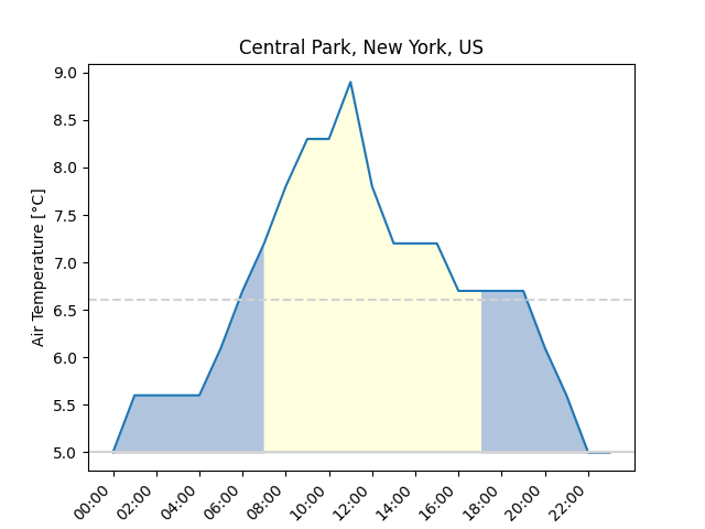
Finally let’s add a horizontal dashed line for the average temperature, a solid line for the minimum temperature and color the area under the graph to indicate day and night hours.

At the observed day and place the actual sunrise was at 07:20 and sunset at 16:38, but for simplicity let us consider the daytime from 07:00 until 17:00.

simple_plot.py

from matplotlib import pyplot
from datetime import datetime, timedelta

start_time = datetime(year=2020, month=12, day=31, hour=0)
air_temperature = [
    5.0, 5.6, 5.6, 5.6, 5.6, 6.1, 6.7, 7.2,
    7.8, 8.3, 8.3, 8.9, 7.8, 7.2, 7.2, 7.2,
    6.7, 6.7, 6.7, 6.7, 6.1, 5.6, 5.0, 5.0
]

minimum_temperature = min(air_temperature)
average_temperature = sum(air_temperature) / len(air_temperature)

hours = [
    start_time + timedelta(hours=offset) 
    for offset in range(len(air_temperature))
]

day_start = 7  # hour index when the first_light shows
day_end = 17   # hour index when the last light fades
daytime = hours[day_start:day_end+1]
daytime_temperature = air_temperature[day_start:day_end+1]
# Last index +1 since we want to include the last hour as endpoint for
# the painted area 

displayed_hours = hours[::2]  # Only display every second hour
displayed_labels = [
    hour.strftime("%H:%M")    # Format as HH:MM
    for hour in displayed_hours
]

pyplot.title("Central Park, New York, US")
pyplot.xlabel("Local time")
pyplot.ylabel("Air Temperature [°C]")
pyplot.xticks(
    ticks=displayed_hours, 
    labels=displayed_labels, 
    rotation=45,
    horizontalalignment="right"  # → from text properties
)

pyplot.plot(hours, air_temperature)

pyplot.axhline(y=average_temperature, linestyle="dashed", color="lightgray")
pyplot.axhline(y=minimum_temperature, linestyle="solid", color="lightgray")
pyplot.fill_between(  # Fill the area below the curve slightly blue
    x=hours, 
    y1=air_temperature, 
    y2=minimum_temperature, 
    color="lightsteelblue"
)
pyplot.fill_between(  # Paint over with yellow for daytime hours
    x=daytime, 
    y1=daytime_temperature, 
    y2=minimum_temperature,
    color="lightyellow"
)

pyplot.show()

Congratulations to your new fancy plot!

Finished plot

Key points¶

Matplotlib uses specific names to describe the elements of a plot
The module pyplot offers shortcuts to quickly generate plots
- It internally keeps track of the current state of the plot that is constructed
- The order in which plotting functions are used, matters
The plot construction is complete when it is shown

Matplotlib Fundamentals

Overview¶

Anatomy of a Plot¶

Creating a simple Plot¶

Example Data¶

The first Steps¶

Adding Details¶

Refinements¶

Decorations¶

Key points¶